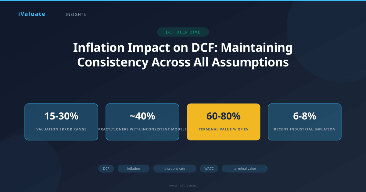
As inflation volatility persists into 2025-2026, with central banks navigating between growth concerns and price stability, corporate valuation professionals face a critical challenge: maintaining internal consistency when inflation assumptions permeate every component of a discounted cash flow (DCF) model. A systematic error in handling nominal versus real cash flows can produce valuation misstatements of 15-30% or more, yet surveys suggest that nearly 40% of practitioners apply inconsistent inflation treatments across their models.

This technical deep dive examines the rigorous framework required to handle inflation correctly in DCF valuations, exploring the mathematical relationships, practical implementation challenges, and common pitfalls that separate sophisticated analysis from flawed work.

01 The Fundamental Framework: Nominal vs. Real Cash Flows

The cornerstone principle is deceptively simple: nominal cash flows must be discounted at nominal rates, while real cash flows must be discounted at real rates. Mixing these frameworks—projecting real cash flows but discounting at nominal rates, or vice versa—creates systematic bias that compounds over the projection period.

The Fisher equation provides the mathematical bridge between nominal and real discount rates:

(1 + nominal rate) = (1 + real rate) × (1 + inflation rate)

Or, in its approximation form for lower rates: nominal rate ≈ real rate + inflation rate

While the approximation works reasonably well at low inflation levels (under 3-4%), the exact Fisher equation becomes essential when dealing with the 4-7% inflation environments we've experienced recently. For example, with a 4% real rate and 6% inflation, the approximation yields 10%, but the exact calculation produces 10.24%—a 24 basis point difference that matters over multi-year projections.

Key Principle: The choice between nominal and real frameworks is ultimately arbitrary for valuation purposes, as mathematically they should yield identical results. However, consistency within the chosen framework is absolutely critical.

02 Revenue Growth: Parsing Volume from Price

Revenue projections represent the first major challenge in inflation-adjusted DCF models. Nominal revenue growth conflates two distinct drivers: volume growth (real expansion of units sold or services delivered) and price inflation. Failing to decompose these components leads to cascading errors throughout the model.

Consider a software-as-a-service company projecting 12% annual revenue growth. If this represents a pure nominal projection in a 5% inflation environment, the implicit real growth is only 6.7% (using the exact Fisher equation: 1.12/1.05 - 1). If the analyst then applies margin assumptions based on historical real performance, or benchmarks against companies reporting in different inflation regimes, the model becomes internally inconsistent.

Practical Implementation Approach

Best practice involves building revenue projections from the ground up:

Volume growth: Project real unit growth based on market expansion, market share gains, and capacity constraints
Price inflation: Apply sector-specific inflation rates, which often differ materially from general CPI
Mix effects: Account for product/service mix shifts that affect average revenue per unit

For a manufacturing business in 2025, this might translate to: 3% volume growth + 4.5% input-cost-driven price increases + 1% favorable mix shift = 8.6% nominal revenue growth. This decomposition becomes essential when projecting margins, as different inflation rates apply to revenue versus costs.

03 Operating Margins: The Inflation Transmission Mechanism

Operating margins represent where inflation assumptions become most complex and where many models fail. The critical insight is that revenue and cost inflation rarely move in lockstep, and the timing of pass-through varies dramatically by business model and competitive position.

Cost Structure Analysis

A rigorous approach requires decomposing the cost base:

Labor costs: Typically inflate at 3-5% in developed markets as of 2025, with wage growth often lagging CPI by 6-12 months
Raw materials: Exhibit higher volatility; industrial commodities showed 6-8% inflation in 2024-2025
Energy: Highly volatile; natural gas and electricity costs for industrial users varied 10-15% year-over-year in recent periods
Rent and occupancy: Generally track CPI with 2-3 year lags due to lease terms

A chemical manufacturer might have a cost structure of 40% raw materials, 25% labor, 15% energy, and 20% other costs. If raw materials inflate at 7%, labor at 4%, energy at 6%, and other costs at 3%, the blended cost inflation is 5.3%—potentially different from both the revenue inflation rate and general CPI.

Pricing Power and Pass-Through Dynamics

The margin trajectory depends critically on pricing power—the ability to pass through cost inflation to customers. This varies by:

Contract structures: Long-term fixed-price contracts create margin compression during inflationary periods
Competitive intensity: Fragmented markets typically allow faster pass-through than concentrated ones
Customer switching costs: High switching costs enable pricing discipline
Product differentiation: Commodity businesses face margin squeeze; differentiated offerings maintain spreads

In practice, most businesses experience a lag between cost inflation and revenue price increases of 2-6 quarters. A DCF model should reflect this timing explicitly. For example, if input costs spike 8% in Year 1 but pricing adjusts only 5% that year and catches up with an additional 3% in Year 2, margins compress temporarily before recovering—a dynamic that materially affects near-term cash flows and thus valuation.

Real-World Example: A specialty chemicals distributor we analyzed in 2024 faced a 9% spike in raw material costs. With 60% of revenue under annual contracts, they could only pass through 4% in Year 1, compressing EBITDA margins from 14% to 11.5%. The DCF needed to model this two-year margin recovery explicitly rather than assuming immediate pass-through.

04 Capital Expenditure: Real Investment vs. Inflation-Driven Replacement

Capital expenditure projections require careful separation of maintenance capex (sustaining current operations) from growth capex (expanding capacity). Inflation affects these differently.

Maintenance Capex

Maintenance capex must inflate at the rate of capital goods inflation, which has run 4-6% annually in recent years for industrial equipment—often above general CPI. A common error is holding maintenance capex constant in nominal terms, which implicitly assumes declining real investment and eventual business deterioration.

The correct approach: establish maintenance capex as a percentage of revenue or as a ratio to depreciation, then inflate both numerator and denominator appropriately. For a manufacturer requiring $10 million annual maintenance capex in Year 1, with capital goods inflating at 5%, Year 5 maintenance capex should be $12.2 million, not $10 million.

Growth Capex

Growth capex projections should reflect the real investment required to support volume growth, inflated by capital goods prices. If a business requires $3 of capex per $1 of incremental revenue in real terms, and revenue grows 3% in real terms with 5% inflation, the nominal growth capex should reflect both the real expansion and the inflation in capital costs.

This becomes particularly important for capital-intensive industries. A data center operator expanding capacity in 2025 faces server and cooling equipment costs inflating at 6-7% while electricity infrastructure costs rise 4-5%. The DCF must model these differential inflation rates on the specific capex components.

05 Working Capital: Often Overlooked, Always Important

Working capital changes represent a subtle but significant inflation challenge. As revenue inflates, so do accounts receivable, inventory, and accounts payable—but at potentially different rates.

Inventory is particularly sensitive. In a FIFO accounting environment with 6% inflation, inventory values increase even with constant unit volumes. If inventory turns are 6x annually (60-day supply), a company with $100 million in revenue needs $16.7 million in inventory. With 6% inflation, maintaining the same 60-day supply requires $17.7 million next year—a $1 million working capital investment that reduces free cash flow.

The rigorous approach models working capital as days of revenue/COGS, then applies appropriate inflation rates to each component. Accounts receivable inflate with revenue (including price inflation), inventory with input costs, and payables with purchase inflation. These rates often differ, creating working capital drags or sources that many models miss.

06 The Discount Rate: WACC in an Inflationary Environment

The discount rate must match the cash flow framework—nominal WACC for nominal cash flows, real WACC for real cash flows. Both the cost of equity and cost of debt require inflation adjustments.

Cost of Equity: CAPM in Nominal Terms

The Capital Asset Pricing Model typically operates in nominal terms:

Cost of Equity = Risk-free rate + Beta × Equity risk premium

The risk-free rate (typically 10-year government bonds) inherently reflects inflation expectations. As of early 2025, 10-year U.S. Treasuries yield approximately 4.3-4.5%, embedding roughly 2.5-2.8% inflation expectations based on TIPS spreads. This represents the nominal risk-free rate.

The equity risk premium (ERP) is more nuanced. Historical ERPs are typically calculated in real terms (6-7% in the U.S. over long periods), but forward-looking ERPs used in practice are usually expressed as nominal premiums over nominal bond yields. Most practitioners use 5.0-6.5% as of 2025, which implicitly includes some inflation compensation.

A critical error occurs when analysts use a real risk-free rate (say, 1.5% from TIPS) plus a nominal ERP (6%), creating an inconsistent 7.5% cost of equity that's neither truly nominal nor real. The correct approach: use nominal Treasury yields (4.3%) plus nominal ERP (5.5-6.0%) for a nominal cost of equity of 9.8-10.3%.

Cost of Debt

Corporate debt costs are inherently nominal—companies borrow and repay in nominal dollars. Current market yields on investment-grade corporate debt range from 5.0-6.5% depending on credit quality, reflecting both real returns and inflation compensation.

For companies with floating-rate debt, inflation affects the cost of debt dynamically through central bank policy responses. As inflation rises, central banks typically increase policy rates, raising floating debt costs. This creates a natural hedge for companies with pricing power (revenues rise with inflation, offsetting higher interest costs) but pressures those unable to pass through inflation.

Calculating Real WACC

If an analyst chooses to work in real terms, the WACC must be deflated consistently. With a nominal WACC of 9.5% and expected inflation of 2.5%, the real WACC is:

Real WACC = (1.095 / 1.025) - 1 = 6.83%

This real WACC would then discount real (inflation-adjusted) cash flows. The mathematical equivalence holds: $100 million nominal cash flow in Year 5 discounted at 9.5% nominal equals $100M / (1.025^5) = $88.4M real cash flow discounted at 6.83% real.

07 Terminal Value: Where Inflation Assumptions Compound

Terminal value typically represents 60-80% of total enterprise value in DCF models, making inflation treatment here absolutely critical. The perpetuity growth method is most sensitive to inflation assumptions.

The Gordon Growth Model

Terminal Value = Final Year FCF × (1 + g) / (WACC - g)

The growth rate 'g' must match the WACC framework. If using nominal WACC, 'g' must be nominal growth. A common error is using a real growth assumption (say, 2-3% real GDP growth) with a nominal WACC, dramatically understating terminal value.

In a 2.5% inflation environment, a 2.5% real perpetuity growth rate translates to approximately 5.1% nominal growth (using Fisher equation: 1.025 × 1.025 - 1). With a 9.5% nominal WACC, this produces:

Terminal Value = FCF × 1.051 / (0.095 - 0.051) = FCF × 23.9x

Using the 2.5% real growth rate incorrectly with the 9.5% nominal WACC would yield FCF × 14.6x—a 39% undervaluation of terminal value.

Exit Multiple Method

The exit multiple approach (applying an EV/EBITDA multiple to terminal year EBITDA) is less obviously affected by inflation but still requires care. The multiple should reflect normalized margins after any inflation-driven compression or expansion has worked through. Using a multiple from a low-inflation period applied to EBITDA in a high-inflation environment can create distortions if margins haven't fully adjusted.

Technical Note: In high-inflation environments (above 5-6%), the perpetuity growth rate approaches or exceeds typical WACC levels, making the Gordon Growth model unstable. In such cases, the exit multiple method or a longer explicit forecast period becomes necessary.

08 Sector-Specific Considerations

Different industries face distinct inflation dynamics that require tailored treatment in DCF models.

Technology and Software

SaaS businesses typically show strong pricing power with minimal cost inflation (labor being the primary cost). Revenue growth often exceeds general inflation by wide margins (10-20%+ nominal growth), while cost bases inflate at 3-5%. This creates natural margin expansion in inflationary environments, which models should capture. However, customer churn may increase if inflation pressures customer budgets.

Consumer Goods

Consumer packaged goods companies face commodity input inflation (often 6-8%) but limited pricing power in competitive retail environments. Models must reflect the 6-12 month lag in price adjustments and potential volume losses from price increases. Private label competition intensifies during inflation, pressuring branded manufacturers.

Real Estate

Real estate valuations are particularly inflation-sensitive. Rental income often includes explicit CPI escalators (2-3% annually), while property values tend to appreciate with inflation over long periods. However, cap rates (the real estate equivalent of discount rates) typically rise with inflation, creating a counterbalancing effect. A real estate DCF should model rental escalations explicitly and use cap rates consistent with the current interest rate environment.

Utilities and Infrastructure

Regulated utilities often have inflation pass-through mechanisms in their rate structures, providing natural inflation protection. However, regulatory lag (the delay between cost increases and rate adjustments) can compress margins temporarily. Infrastructure assets with long-term fixed-price contracts face significant inflation risk, requiring explicit modeling of margin compression.

09 Common Pitfalls and How to Avoid Them

Based on reviews of hundreds of DCF models, several errors recur frequently:

Mixing nominal and real assumptions: The most common error. Solution: Create an explicit inflation assumptions schedule showing the inflation rate applied to each model component.
Using historical margins without inflation adjustment: Historical margins from low-inflation periods don't apply directly in high-inflation environments. Solution: Adjust historical margins for differential revenue vs. cost inflation.
Ignoring working capital inflation: Holding working capital constant in nominal terms. Solution: Model working capital as a percentage of inflating revenue/costs.
Inconsistent terminal value growth: Using real growth rates with nominal WACC. Solution: Always state whether terminal growth is real or nominal and verify consistency.
Static maintenance capex: Failing to inflate replacement costs. Solution: Inflate maintenance capex at capital goods inflation rates.

10 Practical Workflow for Inflation-Consistent DCF Models

A systematic approach ensures consistency:

Establish the framework: Decide whether to work in nominal or real terms (nominal is more common and intuitive for most users)
Document inflation assumptions: Create a dedicated schedule showing inflation rates for revenue, labor costs, material costs, energy, capital goods, and general expenses
Build revenue bottom-up: Separate volume growth from price inflation
Model margins dynamically: Apply different inflation rates to revenue and cost components, reflecting pass-through lags
Inflate capex appropriately: Use capital goods inflation for maintenance capex; model growth capex based on real expansion needs plus inflation
Adjust working capital: Model as days of inflating revenue/costs
Calculate consistent WACC: Ensure risk-free rate, ERP, and debt costs are all nominal (or all real if using real framework)
Verify terminal value: Confirm terminal growth rate matches WACC framework
Sensitivity analysis: Test valuation sensitivity to inflation assumptions, particularly the spread between revenue and cost inflation

11 The Role of Technology in Managing Complexity

The complexity of maintaining inflation consistency across dozens of assumptions and projection years makes sophisticated modeling tools increasingly valuable. Professional platforms like iValuate help practitioners implement these frameworks systematically, with built-in consistency checks that flag mismatches between nominal and real assumptions, automated inflation adjustments across linked schedules, and scenario analysis capabilities that stress-test valuations across different inflation environments.

12 Looking Forward: Inflation Expectations for 2025-2026

As of early 2025, consensus inflation expectations show gradual normalization toward 2.5-3.0% in developed markets, down from the 6-8% peaks of 2022-2023 but above the 2.0% targets most central banks maintain. This creates a transitional environment where:

Historical financial data reflects high-inflation periods that may not repeat
Margin normalization from inflation-driven compression is still working through many businesses
Interest rates remain elevated relative to the 2010s, affecting discount rates
Inflation expectations remain more uncertain than in the previous decade, warranting wider sensitivity ranges

For valuation professionals, this environment demands particular rigor in inflation treatment. The stakes are high: a 1% error in the inflation assumption compounded over a 10-year projection period can shift valuations by 10-15%. In M&A contexts where buyers and sellers negotiate over percentage points of value, these technical details become commercially decisive.

13 Conclusion: Precision as Competitive Advantage

Mastering inflation treatment in DCF models separates sophisticated valuation professionals from those applying rote formulas. As inflation volatility persists and markets adjust to a higher-rate environment than the 2010s, the ability to decompose nominal growth into real and inflationary components, model differential inflation across revenue and cost streams, and maintain rigorous consistency between cash flows and discount rates becomes a source of competitive advantage.

The mathematical framework—rooted in the Fisher equation and the fundamental principle of matching nominal cash flows with nominal discount rates—is straightforward in theory but demanding in practice. It requires detailed understanding of business operations, cost structures, pricing dynamics, and capital requirements. It demands explicit documentation of assumptions and systematic verification of consistency.

For CFOs evaluating strategic alternatives, M&A advisors opining on fairness, private equity professionals underwriting investments, and business owners contemplating liquidity events, getting inflation treatment right in DCF models is not an academic exercise—it's the difference between sound financial decisions and systematic error. Professional tools like iValuate provide the infrastructure to implement these complex frameworks efficiently, allowing practitioners to focus on judgment and insight rather than spreadsheet mechanics, while maintaining the technical rigor that sophisticated valuation demands.

Inflation Impact on DCF: Maintaining Consistency Across All Assumptions