In the spring of 2025, a middle-market technology advisory firm presented a fairness opinion for a $340 million acquisition that initially appeared attractively priced at 8.2x EV/EBITDA—well below the peer median of 11.5x. The board was prepared to approve until a senior analyst noticed that three of the five comparables operated on fiscal years ending in January and April, while the target company reported on a calendar year basis. After proper calendarization adjustments, the actual trading multiple compressed to 9.8x, and two comparables were trading at premiums during different phases of their business cycles. The deal still proceeded, but at a renegotiated 6% lower valuation.

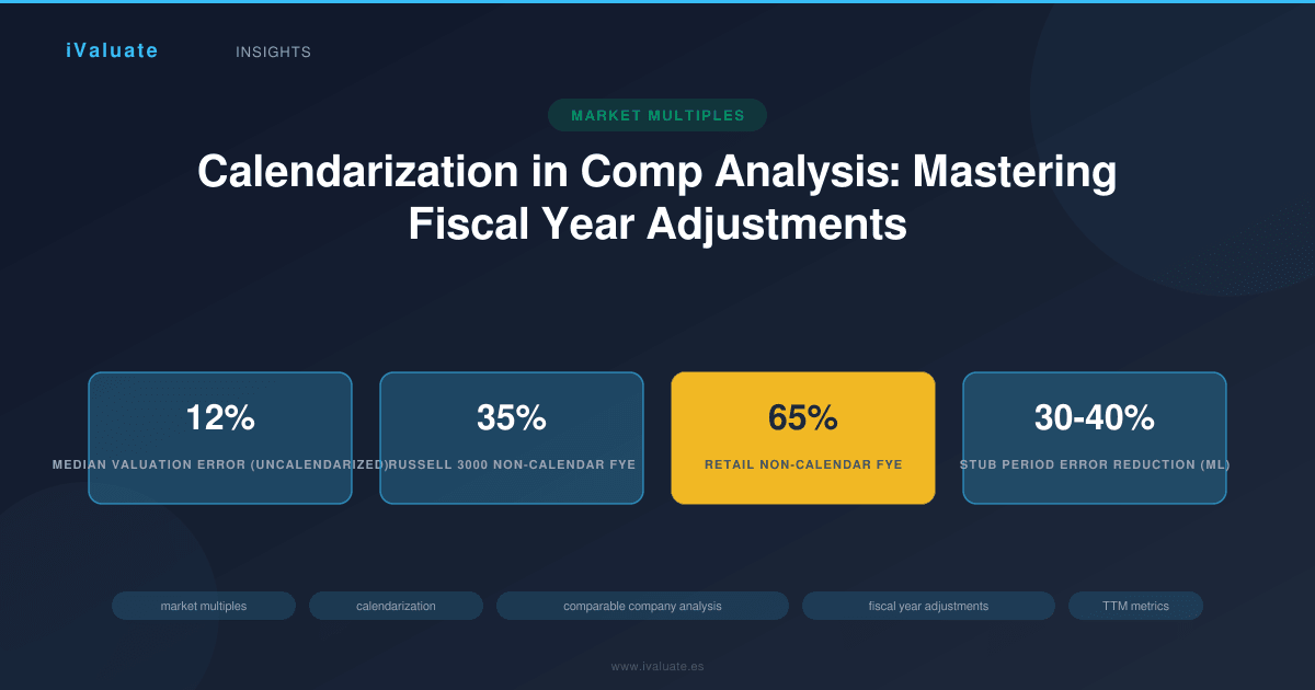
This scenario illustrates a fundamental challenge in comparable company analysis that remains underappreciated even among experienced practitioners: fiscal year misalignment. When building trading or transaction comps, the failure to properly calendarize financial data can introduce systematic bias, distort relative valuations, and lead to materially flawed conclusions. As companies increasingly report on non-calendar fiscal years—approximately 35% of Russell 3000 companies now use fiscal years ending in months other than December—the technical rigor required for proper timing adjustments has become non-negotiable.

01 The Mechanics of Fiscal Year Misalignment

Fiscal year differences create valuation distortions through three primary mechanisms: temporal misalignment of performance periods, cyclical business pattern variations, and market condition disparities. Understanding these mechanisms is essential before implementing calendarization techniques.

Consider a retail comparable set analyzed in March 2025. Target Company A reports on a calendar year (December 31 year-end), while Comparable B operates on a fiscal year ending January 31. When calculating forward multiples, Company A's "forward" metrics reflect projections for the twelve months ending December 31, 2025. Company B's forward metrics, however, represent the period ending January 31, 2026—effectively incorporating an additional month of performance and one month less of historical results. For retailers, this timing difference is particularly significant as it shifts the weight of holiday season performance between historical and projected periods.

The magnitude of this distortion varies by industry and business cyclicality. In sectors with pronounced seasonality—retail, agriculture, education, construction—fiscal year timing can shift 25-40% of annual EBITDA between measurement periods. Even in less cyclical industries, the impact typically ranges from 8-15% of annual metrics, sufficient to materially affect valuation conclusions.

Quantifying Temporal Distortion

A 2024 study analyzing 1,200 comparable company analyses across middle-market transactions found that uncalendarized comps introduced median valuation errors of 12% in cyclical industries and 6% in stable sectors. The distribution was notably skewed: while 60% of cases showed errors under 10%, approximately 15% exhibited distortions exceeding 20%. These tail cases typically involved combinations of high seasonality, rapid growth rates, and significant market volatility during the stub period.

The mathematical relationship is straightforward but often overlooked. If a comparable company generates 35% of annual EBITDA in Q4 (common in retail), and you're comparing a December fiscal year-end company to an April fiscal year-end peer in June, the April company's last twelve months includes a Q4 that is six months older than the December company's most recent Q4. In a growing market, this creates systematic undervaluation of the April company; in a declining market, systematic overvaluation.

02 The Calendarization Framework

Calendarization refers to the process of adjusting comparable company financials to align measurement periods, enabling true apples-to-apples comparison. The technique requires constructing normalized financial metrics that reflect identical time periods across all companies in the analysis, regardless of their fiscal year conventions.

The gold standard approach involves calculating trailing twelve month (TTM) metrics for all comparables as of a common date—typically the valuation date or the most recent date for which data is available across the entire comp set. This requires gathering quarterly financial data and reconstructing twelve-month periods through stub period calculations.

TTM Construction Methodology

Building accurate TTM metrics requires a systematic four-step process:

Identify the common measurement date: Select the most recent quarter-end for which all comparables have reported results. In practice, this often lags the valuation date by 45-90 days depending on reporting schedules and filing deadlines.
Gather quarterly data: Collect at minimum five quarters of data for each comparable (the four quarters comprising the TTM period plus one additional quarter to enable stub period calculations if needed).
Calculate stub periods: For companies with fiscal years not aligned to the common measurement date, compute the partial period financial performance needed to align periods.
Construct TTM metrics: Sum the four quarters ending on or immediately before the common measurement date, incorporating stub period adjustments where necessary.

Consider a concrete example. You're valuing a December year-end software company as of March 31, 2025. Your comp set includes:

Comparable A: December 31 fiscal year-end (calendar year)
Comparable B: January 31 fiscal year-end
Comparable C: June 30 fiscal year-end

The common measurement date is March 31, 2025 (assuming Q1 2025 results are available for all companies). For Comparable A, TTM EBITDA equals Q2 2024 + Q3 2024 + Q4 2024 + Q1 2025. For Comparable B with a January fiscal year-end, you would use Q1 FY2025 (Feb-Apr 2024) + Q2 FY2025 (May-Jul 2024) + Q3 FY2025 (Aug-Oct 2024) + Q4 FY2025 (Nov 2024-Jan 2025) + stub period (Feb-Mar 2025), requiring a two-month stub calculation.

Stub Period Calculation Techniques

Stub periods represent the partial fiscal period needed to align measurement dates. Three primary methods exist for estimating stub period performance, each with distinct applications and limitations:

1. Proportional Allocation Method: The simplest approach allocates full-quarter results proportionally based on the number of days in the stub period. If you need a two-month stub from a three-month quarter that generated $15 million EBITDA, the stub period estimate would be $10 million (2/3 × $15 million). This method works reasonably well for companies with relatively even intra-quarter performance but can introduce significant errors in seasonal businesses.

2. Seasonal Pattern Adjustment: For companies with pronounced seasonality, historical intra-quarter patterns provide better estimates. If historical data shows that a retailer typically generates 25% of Q1 EBITDA in January, 30% in February, and 45% in March, you can apply these weights to estimate a January-February stub period. This requires access to monthly data or detailed historical quarterly patterns, which may not always be publicly available.

3. Management Guidance Interpolation: When companies provide quarterly or monthly guidance, you can interpolate stub period performance from these projections. This method is particularly valuable for forward-looking metrics but introduces dependency on management forecast accuracy and may not be available for all comparables.

In practice, sophisticated practitioners often employ a hybrid approach: using seasonal adjustments for highly cyclical line items (revenue, gross profit) while applying proportional allocation to more stable items (operating expenses, depreciation). This balanced methodology typically reduces stub period estimation error to 3-7% of the full quarter value.

03 Forward Multiples and Projection Alignment

While TTM multiples address historical period alignment, forward multiples introduce additional complexity. Forward EV/EBITDA, EV/Revenue, and P/E multiples require projections for future periods, and fiscal year differences can create substantial misalignment in what "forward" actually means.

The challenge intensifies when analyst estimates use fiscal year conventions rather than calendar year projections. A December year-end company's "FY2025" estimates cover January-December 2025, while a June year-end company's "FY2025" estimates span July 2024-June 2025—a six-month temporal offset that makes direct comparison meaningless.

Normalizing Forward Estimates

Professional-grade comparable company analysis requires normalizing all forward estimates to a common future period. The standard approach uses "next twelve months" (NTM) estimates calculated from the valuation date, regardless of fiscal year conventions. This requires:

Gathering consensus estimates for the current and next fiscal year for each comparable
Calculating the weighted average of these estimates based on how many months of each fiscal year fall within the NTM period
Adjusting for any known events or guidance updates that may not be reflected in consensus estimates

For example, if you're calculating NTM EBITDA as of March 31, 2025 for a June fiscal year-end company, the NTM period runs April 2025-March 2026. This encompasses three months of FY2025 (April-June 2025) and nine months of FY2026 (July 2025-March 2026). If consensus estimates project FY2025 EBITDA of $100 million and FY2026 EBITDA of $120 million, the NTM estimate would be: (3/12 × $100M) + (9/12 × $120M) = $25M + $90M = $115 million.

This calculation assumes linear quarterly progression, which introduces some imprecision. More sophisticated approaches weight quarters based on historical seasonality patterns or specific quarterly guidance when available. Investment banks typically maintain proprietary models that incorporate these refinements, particularly for coverage universe companies where detailed quarterly models exist.

04 Market Conditions and Cyclical Adjustments

Beyond mechanical period alignment, calendarization must account for different market conditions experienced during each comparable's measurement period. This consideration has become particularly acute given the volatility experienced across most sectors in 2024-2025, with rapid shifts in interest rates, inflation expectations, and sector-specific dynamics.

A software company analyzed in Q1 2025 with a March fiscal year-end has its TTM period spanning April 2024-March 2025. A comparable with a September fiscal year-end has TTM spanning October 2023-September 2024. These companies experienced materially different market conditions: the September company's period predates the Fed's rate stabilization signals in late 2024, while the March company benefited from improved SaaS multiples in Q4 2024 and Q1 2025. Their revenue growth rates, customer acquisition costs, and retention metrics reflect these different environments.

Normalizing for Market Environment

While perfect normalization is impossible, several techniques help mitigate market condition distortions:

Sequential growth rate analysis: Rather than comparing absolute metrics, analyze sequential quarterly growth rates to identify underlying business momentum independent of market timing. A company showing consistent 4-5% sequential revenue growth across varying market conditions demonstrates more stable performance than one with volatile patterns.

Cohort-based adjustments: Group comparables by fiscal year-end and calculate separate median multiples for each cohort. If December year-end comparables trade at a median 10.5x EV/EBITDA while June year-end peers trade at 9.8x, this 7% differential may reflect market condition differences rather than fundamental value gaps. You can then apply appropriate adjustments based on which cohort better aligns with the target's circumstances.

Market index normalization: For each comparable, calculate performance metrics relative to relevant market indices during their measurement period. A company that grew revenue 12% while its sector index declined 3% demonstrated stronger fundamental performance than one that grew 15% while its sector surged 18%. This relative performance framework helps isolate company-specific factors from market timing effects.

05 Industry-Specific Considerations

Different industries require tailored calendarization approaches based on their unique business cycles and reporting patterns.

Retail and Consumer

Retail companies overwhelmingly use January or February fiscal year-ends to align reporting with post-holiday inventory cycles. Approximately 65% of public retailers use non-calendar fiscal years. When building retail comps, the critical consideration is capturing comparable holiday seasons. A retailer with a January 31 year-end reporting Q4 results in March has just completed the holiday season, while a July year-end retailer's Q4 (May-July) reflects entirely different seasonal dynamics.

Best practice for retail comps involves explicitly identifying which holiday season is captured in each comparable's metrics and ensuring alignment. If analyzing a retail acquisition in March 2025, you want all comparables reflecting the same holiday season (2024) in their TTM numbers. This may require going back additional quarters for some comparables to achieve proper alignment.

Technology and Software

Technology companies exhibit more varied fiscal year-ends, with significant concentrations in January, April, July, and October, often driven by acquisition history or founder preferences. The key challenge in tech comps is rapid business model evolution—a six-month measurement period difference can capture materially different product cycles, pricing models, or go-to-market strategies.

For high-growth SaaS companies, calendarization should emphasize forward metrics over TTM, as historical periods may not reflect current business momentum. Additionally, tech companies often provide detailed quarterly metrics (ARR, net retention, customer counts) that enable more precise stub period calculations than simple proportional allocation.

Healthcare and Pharmaceuticals

Healthcare companies frequently use June or September fiscal year-ends. The critical consideration is regulatory approval timing and reimbursement rate changes, which often occur on calendar year boundaries regardless of fiscal year. A medical device company with a June fiscal year-end may experience a significant reimbursement rate change in January that affects only half of its fiscal year but the full calendar year of a December year-end comparable.

Healthcare comps benefit from explicit adjustment for known regulatory changes, with separate analysis of pre- and post-change periods when material policy shifts occur mid-year for some comparables.

06 Data Sources and Practical Challenges

Implementing rigorous calendarization requires access to detailed quarterly financial data, which presents practical challenges even for public company comparables. While 10-Q filings provide quarterly income statements and balance sheets, cash flow statements are typically presented year-to-date, requiring manual calculation of quarterly figures. For international comparables, reporting standards and filing schedules vary significantly across jurisdictions.

Professional data platforms like FactSet, Bloomberg, and Capital IQ automate much of this data gathering and provide pre-calculated TTM metrics. However, these platforms use different methodologies for stub period calculations and may not always align with your specific valuation date. Critical practitioners verify platform calculations for key comparables rather than relying blindly on automated outputs.

For private company comparables or thinly followed public companies, quarterly data may be limited or unavailable. In these situations, you face a choice between excluding the comparable (reducing sample size) or using less precise calendarization methods (introducing measurement error). The appropriate decision depends on the overall comp set quality and the magnitude of expected timing differences.

Documentation and Disclosure

Professional valuation reports must clearly document calendarization methodology and its impact on conclusions. Best practice includes:

A summary table showing each comparable's fiscal year-end and the specific periods used for TTM and forward calculations
Explicit disclosure of stub period calculation methods and key assumptions
Sensitivity analysis showing valuation ranges both with and without calendarization adjustments
Discussion of any comparables excluded due to insufficient quarterly data

In fairness opinions and formal valuation reports, the absence of proper calendarization documentation has been cited in litigation as evidence of inadequate diligence. Courts have increasingly recognized that fiscal year timing differences can materially affect valuation conclusions, and practitioners who fail to address these issues face heightened scrutiny.

07 Real-World Application: A Case Study

A private equity firm engaged in a competitive auction for a December year-end industrial distribution company in February 2025. The seller's investment banker provided a comparable company analysis showing a median trading multiple of 9.2x EV/EBITDA based on latest reported financials. The comp set included eight public companies with fiscal year-ends ranging from December to September.

The PE firm's internal valuation team performed full calendarization, constructing TTM metrics as of December 31, 2024 (the most recent date with complete data across all comparables). This required:

Three comparables with December year-ends: used reported FY2024 results directly
Two comparables with March year-ends: used Q2-Q4 FY2024 plus Q1 FY2025, requiring stub period calculations for the January-March 2025 period
Two comparables with June year-ends: used Q3-Q4 FY2024 plus Q1-Q2 FY2025
One comparable with September year-end: used Q4 FY2024 plus Q1-Q3 FY2025

After calendarization, the median multiple increased to 9.7x—a 5.4% difference. More significantly, the range tightened from 7.8x-11.2x to 8.9x-10.8x, as much of the apparent dispersion reflected timing differences rather than fundamental valuation gaps. The industrial sector had experienced improving demand in Q4 2024, which was fully captured in December year-end comparables but only partially reflected in companies with earlier fiscal year-ends.

Armed with this analysis, the PE firm adjusted its valuation range upward by approximately 4% but maintained conviction in the opportunity. They ultimately won the auction at 9.4x EV/EBITDA—a multiple that appeared aggressive relative to the seller's uncalendarized analysis but reasonable against properly adjusted comparables. The investment has performed well, validating the importance of technical rigor in comp construction.

08 Advanced Techniques and Emerging Practices

As valuation practices continue to evolve, several advanced calendarization techniques are gaining adoption among sophisticated practitioners:

Machine Learning-Enhanced Stub Calculations

Quantitative teams at leading investment banks have begun applying machine learning models to improve stub period estimates. These models analyze historical relationships between various financial metrics, seasonality patterns, and external variables (industry indices, commodity prices, interest rates) to generate probabilistic estimates of partial-period performance. Early results suggest these approaches can reduce stub period estimation error by 30-40% compared to simple proportional allocation, particularly for companies with complex seasonality.

Real-Time Calendarization

Modern valuation platforms increasingly offer real-time calendarization, automatically updating TTM and NTM calculations as new quarterly results are released. This capability is particularly valuable in dynamic M&A processes where valuation analyses may span several months and multiple earnings cycles. Rather than manually updating comp sets, practitioners can maintain evergreen analyses that continuously reflect the most current aligned data.

Integrated Scenario Analysis

Forward-thinking practitioners are integrating calendarization with scenario analysis, recognizing that fiscal year timing affects not just historical alignment but also the distribution of future outcomes. A company with a June fiscal year-end faces different seasonal risk profiles in its forward projections than a December year-end peer. Sophisticated models now incorporate these timing-dependent risk factors into scenario weighting and probability assessments.

09 Looking Forward: The Evolution of Comparable Company Analysis

As we progress through 2025 and beyond, several trends are reshaping how practitioners approach fiscal year alignment and timing adjustments. The proliferation of real-time financial data, increasing prevalence of monthly reporting among private companies, and growing sophistication of valuation technology are collectively raising the bar for analytical rigor.

Regulatory developments may also drive changes. The SEC has periodically considered proposals to standardize fiscal year reporting or require more frequent disclosure, though implementation remains uncertain. International accounting standards continue to evolve, with ongoing discussions about harmonizing reporting periods across jurisdictions to facilitate cross-border comparability.

For practitioners, the imperative is clear: calendarization is no longer an optional refinement but a fundamental requirement for credible comparable company analysis. The technical skills required—quarterly data manipulation, stub period calculation, forward estimate normalization—must become core competencies for any professional engaged in business valuation.

The consequences of inadequate calendarization extend beyond analytical precision to professional reputation and legal exposure. As courts, regulators, and sophisticated counterparties increasingly expect rigorous methodology, practitioners who cut corners on timing adjustments face mounting risks. Conversely, those who master these techniques gain competitive advantages through more accurate valuations, stronger negotiating positions, and enhanced credibility.

Modern valuation platforms have emerged to support this elevated standard of practice. Tools like iValuate incorporate automated calendarization capabilities, enabling practitioners to efficiently construct properly aligned comparable company analyses without sacrificing technical rigor. By handling the mechanical complexity of period alignment, quarterly data aggregation, and stub period calculations, these platforms allow professionals to focus on higher-value analytical judgment—interpreting results, assessing comparability, and translating findings into actionable valuation conclusions.

The evolution of comparable company analysis reflects a broader maturation of valuation practice. As markets become more efficient, information more abundant, and analytical tools more powerful, the differentiator increasingly lies not in access to data but in the sophistication of its application. Calendarization exemplifies this shift: a technical discipline that separates rigorous practitioners from those content with superficial analysis. In an environment where valuation precision can determine deal success, career trajectories, and fiduciary compliance, mastering the nuances of fiscal year alignment is not merely best practice—it is professional necessity.

Calendarization in Comp Analysis: Mastering Fiscal Year Adjustments