APV vs WACC-Based DCF: When Adjusted Present Value Delivers Superior Results

In the evolving landscape of corporate valuation, the debate between Adjusted Present Value (APV) and traditional Weighted Average Cost of Capital (WACC) approaches continues to shape how sophisticated investors and advisors value complex transactions. While WACC-based discounted cash flow remains the workhorse of valuation practice, the APV method offers distinct advantages in scenarios where capital structure changes significantly or financing effects require explicit modeling.

As we navigate the high-interest-rate environment of 2025-2026, with benchmark rates stabilizing between 4.5% and 5.5%, the choice between these methodologies has taken on renewed importance. The explicit separation of operating and financing effects in APV provides clarity that proves invaluable in leveraged transactions, restructurings, and project finance—contexts where traditional WACC assumptions break down.

01 Understanding the Fundamental Difference

The traditional WACC approach values a company by discounting free cash flows at a blended cost of capital that reflects the target capital structure. This single discount rate embeds both the operating risk of the business and the financial risk from leverage. The formula is deceptively simple:

Where E represents equity value, D represents debt value, V is total firm value, Re is the cost of equity, Rd is the cost of debt, and Tc is the corporate tax rate. The method assumes a constant capital structure maintained at target levels—an assumption that often proves unrealistic.

The APV method, by contrast, separates the valuation into distinct components:

• The unlevered firm value (operating assets discounted at the unlevered cost of equity)
• The present value of financing side effects (primarily the tax shield from debt)
• Other financing benefits or costs (such as subsidized financing or financial distress costs)

This separation allows analysts to model each component with appropriate assumptions and discount rates, providing both transparency and flexibility that WACC cannot match.

02 When APV Demonstrates Clear Superiority

Leveraged Buyouts and Recapitalizations

In leveraged buyout scenarios, where private equity sponsors typically plan aggressive debt paydown schedules, the capital structure changes dramatically over the investment horizon. A recent middle-market LBO in the software sector illustrates this perfectly: the sponsor acquired the target with 5.5x debt-to-EBITDA leverage in early 2025, planning to reduce this to 2.0x by year five through cash flow generation.

Using WACC in this context requires either:

• Calculating a different WACC for each year (computationally intensive and conceptually muddled)
• Using an average WACC (which misrepresents the actual cost of capital in any given year)
• Assuming constant leverage (which contradicts the business plan)

APV elegantly sidesteps these issues. The analyst values the unlevered cash flows at a constant unlevered cost of equity (typically 12-14% for middle-market software companies in current markets), then separately values the declining tax shields as debt pays down. This approach captured an additional $47 million in value compared to a simplified constant-WACC approach—a 6.8% difference in enterprise value that proved material to the investment decision.

Project Finance and Infrastructure Investments

Infrastructure projects and project finance structures represent another domain where APV excels. These investments typically feature:

• High initial leverage (often 70-80% debt-to-total capital)
• Contractual debt amortization schedules
• Predictable cash flows with limited reinvestment needs
• Potentially subsidized or below-market financing from development banks

Consider a renewable energy project financed in 2025 with $400 million in senior debt at 6.2% (market rate) and $100 million in subordinated debt from a green development bank at 3.8% (below market rate). The APV framework allows explicit valuation of this financing subsidy—worth approximately $18 million in present value terms—that would be obscured in a WACC calculation.

Distressed and Turnaround Situations

When companies face financial distress, the relationship between leverage and firm value becomes nonlinear. The costs of financial distress—including restricted operations, customer attrition, supplier constraints, and potential bankruptcy costs—must be explicitly modeled. APV provides the framework to do this.

In a 2024 retail restructuring, the company carried $280 million in debt against an enterprise value that had declined to approximately $320 million, implying a debt-to-value ratio exceeding 85%. The probability of distress was material, with estimated distress costs of $45-60 million. The APV approach allowed the advisory team to:

• Value the unlevered business based on restructured operations
• Add the present value of tax shields (limited by the probability of generating taxable income)
• Subtract the probability-weighted costs of financial distress

This granular approach supported negotiations that ultimately preserved $95 million in stakeholder value compared to a liquidation scenario.

03 The Miles-Ezzell Adjustment: Precision in Tax Shield Valuation

A critical technical consideration in APV implementation involves how to discount the tax shields. The naive approach discounts tax shields at the cost of debt, assuming they're as risky as the debt that generates them. However, this assumption only holds if the firm maintains a constant dollar amount of debt.

Most companies instead target a leverage ratio—maintaining debt as a percentage of firm value. This creates a subtle but important difference: as firm value fluctuates, so does the debt level, making tax shields riskier than the debt itself. Miles and Ezzell (1980) derived the correct adjustment for this scenario.

Under the Miles-Ezzell framework, when a company maintains constant leverage (debt as a percentage of value), the tax shield in year t should be discounted as:

PV(Tax Shield) = [Tc × Rd × D₀] / (1 + Rd) + Σ [Tc × Rd × Dt] / (1 + Ru)^t

Where the first year's tax shield is discounted at the cost of debt (Rd), but subsequent shields are discounted at the unlevered cost of equity (Ru). This reflects that future tax shields depend on future firm value, which is uncertain.

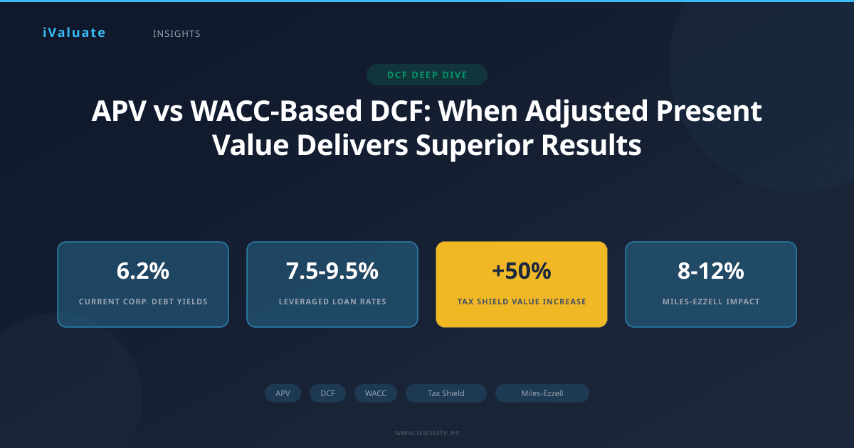
The practical impact is meaningful. For a company with $500 million in debt, a 6.5% cost of debt, 24% tax rate, and 11% unlevered cost of equity, the Miles-Ezzell approach yields a tax shield value approximately 8-12% lower than the simpler approach of discounting all shields at the cost of debt. In absolute terms, this represents $15-20 million in valuation difference—material in any transaction context.

Implementation in Practice

Implementing Miles-Ezzell correctly requires:

1. Clear identification of the leverage policy: Does management target constant dollar debt or constant leverage ratio? Interview management and review historical patterns.
2. Appropriate discount rate selection: Use the cost of debt for the first period's shield, then the unlevered cost of equity for subsequent periods if leverage is maintained as a ratio.
3. Consistency checks: Verify that the implied levered cost of equity from your APV matches what you'd calculate using the Modigliani-Miller propositions with taxes.

In the current environment, where debt costs have risen sharply from the 2020-2021 lows, the tax shield component has become more valuable. A company with $300 million in debt refinanced in 2025 at 7.0% (versus 3.5% in 2021) generates annual tax shields of $5.04 million (at a 24% tax rate) compared to $2.52 million previously—exactly double. This makes precise tax shield valuation more important than ever.

04 Calculating the Unlevered Cost of Equity

The foundation of APV is the unlevered cost of equity—the return required by equity investors if the company had no debt. This represents the pure business risk without financial leverage. Three primary methods exist for estimation:

Method 1: Unlevering Observed Equity Betas

Start with the observed levered beta of the company (or comparable companies), then unlever using the Hamada formula:

βu = βL / [1 + (1 - Tc) × (D/E)]

For a software company with a levered beta of 1.35, debt-to-equity ratio of 0.40, and 24% tax rate, the unlevered beta would be 1.09. With a risk-free rate of 4.8% and equity risk premium of 6.5% (consensus estimates for 2025), the unlevered cost of equity is 11.9%.

Method 2: Build-Up Approach

For private companies or divisions without observable betas, construct the unlevered cost of equity from components:

• Risk-free rate: 4.8% (10-year Treasury as of early 2025)
• Size premium: 2.5-4.0% (depending on company size)
• Industry risk premium: 1.5-3.5% (varying by sector volatility)
• Company-specific risk: 0-2.0% (for idiosyncratic factors)

A middle-market industrial distributor might warrant: 4.8% + 3.2% + 2.1% + 1.0% = 11.1% unlevered cost of equity.

Method 3: Reverse Engineering from Transaction Multiples

When recent transactions exist, work backwards from observed multiples to implied returns. If comparable companies trade at 8.5x EV/EBITDA and generate EBITDA margins of 18% with modest growth, this implies unlevered returns in the 10-12% range after accounting for reinvestment needs.

05 Comprehensive APV Example: Manufacturing Acquisition

Consider a detailed example: a strategic buyer evaluating a specialty manufacturing company in Q1 2025. The target generates $85 million in EBITDA with expectations for 4% annual growth. The acquisition will be financed with $400 million in debt (4.7x leverage) at 7.25%, with planned paydown to $200 million over seven years.

Step 1: Calculate Unlevered Free Cash Flows

Project EBITDA, subtract taxes on EBIT (at 24% rate), add back depreciation, subtract capex and working capital needs. This yields unlevered FCF starting at $48 million in year one, growing to $61 million by year seven.

Step 2: Determine Unlevered Cost of Equity

Comparable public companies show levered betas averaging 1.15 with debt-to-equity ratios of 0.35. Unlevering yields βu = 0.93. With Rf = 4.8% and ERP = 6.5%, the unlevered cost of equity is 10.8%.

Step 3: Value Unlevered Firm

Discounting the unlevered FCF at 10.8% and applying a terminal value (using a perpetuity growth rate of 2.5%), the unlevered enterprise value is $687 million.

Step 4: Value Tax Shields

With debt declining from $400M to $200M, annual interest expense falls from $29M to $14.5M, generating tax shields from $7.0M to $3.5M. Using Miles-Ezzell, discount the first year at 7.25% and subsequent years at 10.8%. The present value of tax shields totals $38 million.

Step 5: Consider Other Effects

The buyer identifies $12 million in integration costs (present value) and expects $8 million in present value from utilizing the target's NOLs. Net adjustment: -$4 million.

Total APV: $687M + $38M - $4M = $721 million

By comparison, a traditional WACC approach using a blended rate (calculated at various points in the debt paydown schedule) yielded values ranging from $695M to $738M depending on assumptions—a range that created uncertainty in negotiations. The APV's transparency allowed the buyer to understand exactly where value originated and supported a final purchase price of $710 million.

06 Common Pitfalls and How to Avoid Them

Pitfall 1: Inconsistent Tax Treatment

Analysts sometimes calculate unlevered FCF using the actual tax paid (which reflects interest deductions) rather than the tax on unlevered earnings. This double-counts the tax benefit of debt. Always calculate unlevered FCF using taxes on EBIT without interest deductions—the tax shield is captured separately.

Pitfall 2: Wrong Discount Rate for Tax Shields

As discussed, blindly discounting all tax shields at the cost of debt overstates their value when leverage is maintained as a ratio rather than a fixed dollar amount. Apply Miles-Ezzell when appropriate.

Pitfall 3: Ignoring Debt Capacity Constraints

APV can theoretically suggest that more leverage always adds value (through tax shields). In reality, debt capacity is limited by cash flow coverage, covenant restrictions, and distress costs. Always sanity-check that implied leverage ratios remain within reasonable bounds for the industry and company size.

Pitfall 4: Circular References in Modeling

When debt is defined as a percentage of firm value, and firm value includes the value of tax shields, which depend on debt levels, a circular reference emerges. Sophisticated models require iterative calculations or simultaneous equation solving. Most practitioners resolve this by either:

• Using Excel's iterative calculation feature (with appropriate convergence settings)
• Fixing debt levels based on the unlevered value plus a reasonable estimate of tax shield value
• Employing specialized valuation software that handles these calculations automatically

07 APV in the Current Market Environment

The elevated interest rate environment of 2025-2026 has made APV particularly relevant. With the Federal Reserve maintaining benchmark rates in the 4.5-5.5% range to ensure inflation remains controlled, corporate borrowing costs have settled at levels not seen since 2007-2008. Investment-grade corporate debt yields average 6.2%, while leveraged loan rates for sponsor-backed deals range from 7.5-9.5% depending on credit quality.

This environment creates several implications for APV analysis:

Higher tax shield values: With debt costs elevated, the absolute dollar value of tax shields has increased proportionally. A company with $500 million in debt paying 7.5% interest generates $9 million in annual tax shields (at 24% tax rate) versus $6 million when rates were 5.0%. Over a ten-year horizon, this difference compounds to $25-30 million in additional present value.

Greater scrutiny of leverage sustainability: Higher debt costs mean tighter coverage ratios. APV's explicit modeling of debt levels over time helps identify when leverage becomes unsustainable. In several 2024-2025 transactions, APV analysis revealed that planned debt levels would violate 2.0x interest coverage covenants by year three, forcing deal restructuring.

Increased value of rate hedging: Many sponsors now incorporate interest rate swaps or caps into their financing structures. APV provides a natural framework to value these instruments separately, adding their value (or cost) as distinct components rather than trying to embed them in a WACC calculation.

08 Software and Tools for APV Implementation

While APV can be implemented in Excel, the circular references and iterative calculations required for precision make specialized tools valuable. Professional valuation platforms have evolved to handle these complexities, automatically solving for consistent debt levels, tax shields, and firm values while maintaining Miles-Ezzell adjustments.

The key features to look for in APV-capable tools include:

• Flexible debt schedule inputs (both dollar amounts and leverage ratios)
• Automatic Miles-Ezzell adjustments with user override options
• Sensitivity analysis across multiple variables simultaneously
• Clear audit trails showing how each value component is calculated
• Integration with market data for cost of capital inputs

These capabilities become particularly valuable in complex situations involving multiple debt tranches, changing tax rates, or international structures with varying tax regimes.

09 Looking Forward: APV in an Evolving Valuation Landscape

As we progress through 2025 and into 2026, several trends suggest APV will become increasingly important in valuation practice:

Private credit growth: The expansion of private credit markets has created more diverse and complex financing structures. Direct lenders often provide unitranche facilities with embedded PIK toggles, equity kickers, or other features that are difficult to capture in a single WACC. APV's component-based approach handles this complexity naturally.

ESG-linked financing: Sustainability-linked loans and green bonds offer interest rate step-downs tied to ESG metrics. These contingent financing benefits are best valued explicitly in an APV framework rather than trying to estimate an average WACC.

Cross-border complexity: With increasing global M&A activity, deals often involve multiple tax jurisdictions with different rates and rules. APV allows separate modeling of tax shields in each jurisdiction, providing accuracy that blended WACC approaches cannot achieve.

Regulatory scrutiny: Regulators and courts increasingly demand transparency in valuation methodologies, particularly in fairness opinions and solvency analyses. APV's explicit separation of operating and financing effects provides the clarity that withstands scrutiny.

10 Conclusion: Choosing the Right Tool for the Job

The choice between APV and WACC-based DCF is not about which method is universally superior—both have their place in the valuation toolkit. WACC remains efficient and appropriate for stable companies with relatively constant capital structures and straightforward financing. Its simplicity and widespread acceptance make it the default choice for many valuations.

However, when capital structure changes significantly, when financing effects require explicit modeling, or when transparency is paramount, APV demonstrates clear superiority. The method's ability to separately value operating performance, tax shields, and other financing effects provides both precision and insight that WACC cannot match.

For professionals navigating today's complex deal environment—with elevated interest rates, diverse financing structures, and increasing scrutiny—mastering APV implementation is no longer optional. The technical rigor required, from proper unlevering of betas to correct application of Miles-Ezzell adjustments, demands both theoretical understanding and practical experience.

Modern valuation platforms like iValuate have made sophisticated APV analysis more accessible, handling the computational complexity while maintaining the transparency that makes the method valuable. As deal structures continue to evolve and financing becomes more creative, the analysts and advisors who can fluently apply both WACC and APV—choosing the right tool for each situation—will deliver the most accurate and defensible valuations.

The question is not whether to learn APV, but rather how quickly you can incorporate it into your valuation practice. In an environment where a 5-10% valuation difference can determine whether a deal proceeds or collapses, the precision that APV provides is not merely academic—it's essential to making sound investment decisions.